Planet

Planet is San Francisco based company who operates a fleet of small imaging satellites. Their aim is to provide daily, high-resolution, coverage of the entire globe. Their “Dove” cubesats image in 4 channels (blue, green, red, and NIR) with a resolution of up to 3m (I think they are trying to get this even lower). They sell access to their data for most of the globe, but provide free access for data within California via their Open California initiative.

This post is a brief description of how I went about accessing some of their data, mainly following this guide and this example.

Accessing the data

Planet has available a browser based interactive tool that allows you to browse imagery over the globe in both location and time and then (depending on your access level) download the data. I was more interested in accessing it programmatically via their API so I signed up and got myself an API key!

They provide both command line access to the API, and have Python and java clients. I’m going to use the Python client for this post.

The Planet API client is imported into python and a client instance is launched like this:

from planet import api
from planet.api import filters

# will pick up api_key via environment variable PL_API_KEY
# creates a client instance
client = api.ClientV1()

The data is accessed querying the API with a spatial, temporal, and product filter. A long time ago, I worked as a liftie at Kirkwood Mountain Resort, just south of South Lake Tahoe in the Sierra-Nevadas so I figured that’d make a good location within California to examine.

The geometry filter requires a geoJSON object, which I generated using geojson.io giving me this polygon and code (after some small modifications)

aoi = {
  "type": "Polygon",
  "coordinates": [
    [
      [
        -120.07713317871094,
        38.70721396458306
      ],
      [
        -120.09653091430663,
        38.68644773215067
      ],
      [
        -120.06185531616211,
        38.66299474019031
      ],
      [
        -120.03335952758788,
        38.681489740151555
      ],
      [
        -120.051212310791,
        38.703061200438505
      ],
      [
        -120.07713317871094,
        38.70721396458306
      ]
    ]
  ]
}

The query filter is constructed by providing the geometry filter, a date range filter, and a range_filter which I’m using to specify the cloud cover limits (I think it can be used to specify other limits as well but couldn’t find any more documentation).

# build a query using the AOI,
# a cloud_cover filter, and a date range
query = filters.and_filter(
    filters.geom_filter(aoi),
    filters.range_filter('cloud_cover', lt=0.25),
    filters.date_range('acquired', gt="2016-11-01T00:00:00.000Z",
                         lt='2017-01-01T00:00:00.000Z'),
)

The next step is too specify the product you want, the options are:

PSScene3Band:	PlanetScope Scenes with only RGB bands
PSScene4Band:	PlanetScope Scenes with all 4 bands
PSOrthoTile:	PlanetScope OrthoTiles
REOrthoTile:	RapidEye OrthoTiles
REScene:	RapidEye Scenes (unorthorectified strips)
Landsat8L1G:	Landsat8 Scenes
Sentinel2L1C:	Copernicus Sentinel-2 Scenes

PlanetScope is data from the Planet Lab satellites, Rapid Eye comes from another commercial satellite data provider that Planet Lab acquuired in 2015. Landsat is the NASA/USGS instrument, and Sentinel-2 is the ESA instrument. For this post I’m using the PSScene4Band dataset.

request = filters.build_search_request(
    query, item_types=['PSScene4Band']
)

You then perform the search

results = client.quick_search(request)

You can then download the data that matches your search query by iterating of the results items. Each item has to be activated on the API endpoint before it can be downloaded.

# loop over the results returned by the query (just doing one here)
for item in results.items_iter(1):
    #
    assets = client.get_assets(item).get()
    # analytic is the data, analytic_xml contains metadata
    for asset in ['analytic', 'analytic_xml']:

        # The requested item must be activated on the API, this can take a few mins
        activation = client.activate(assets[asset])

        # wait for activation
        while assets[asset]['status'] != 'active':
            time.sleep(30)

            assets = client.get_assets(item).get()

        # Once the item is active we can download it
        callback = api.write_to_file(directory='/Users/joe/dev_work/planet/images')
        body = client.download(assets[asset], callback=callback)
        body.await()

Using the GDAL python library and a nice package called Spectral Python we can load and view the downloaded file (note the band order).

import numpy as np
from spectral import imshow
import gdal

ds = gdal.Open('../images/20161229_211150_0c60_3B_AnalyticMS.tif')

blue = ds.GetRasterBand(1).ReadAsArray()
green = ds.GetRasterBand(2).ReadAsArray()
red = ds.GetRasterBand(3).ReadAsArray()
nir = ds.GetRasterBand(4).ReadAsArray()

img = np.dstack((red, green, blue))

imshow(img, stretch=0.05)

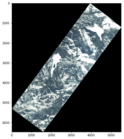
And we see some nice looking snowy mountains!

In my next post for this I’m going to look in more depth at the actual data.